Simple Guidance Mechanisms for Discrete Diffusion project page

Guidance + Diffusion👌

State-of-the-art diffusion models are the prevailing approach for generating continuous signals, such as images and audio. These models are made even more useful by the mechanisms of classifier-free and classifier-based guidance that enable users to better control the generated samples. In contrast, for discrete data, autoregressive (AR) models are the go-to approach, but are notoriously difficult to control, given the sequential nature of their generation process that 'locks in' tokens during denoising. Diffusion models, which have a global view of a generated signal at each denoising step, as opposed to AR models which can only plan locally (i.e., one token ahead), are arguably more suitable for controlled generation. Finding a way to bridge the gap to AR's language modeling performance while maintaining the control mechanisms of diffusion modeling would unlock powerful and useful generative modeling tools with widespread applications, especially in scientific domains.

Recent work on discrete diffusion (e.g., Sahoo et al., 2024) poses a potential alternative to AR language modeling. The improved performance of non-autoregressive language models inspires a renewed search for guidance mechanisms that, similar to the continuous domain, can unlock high-quality controllable generation for discrete data.

Our contributions

We provide simple and effective discrete classifier-based and classifier-free guidance.
We introduce UDLM, a class of discrete diffusion models particularly amenable to guidance, and we derive a tightened ELBO that significantly improves their performance.
Across three domains, we demonstrate that discrete guidance yields better controllable generation compared to strong AR baselines and previous diffusion guidance methods.

Discrete Diffusion Models (a brief primer)

In diffusion, we train a parametric model $p_\theta$ to undo corruption from latent variables $\mathbf{z}_t$ (for $t \in [0, 1]$) that are produced from a fixed forward noising process defined by $q$ (Sohl-Dickstein et al., 2015; Song & Ermon, 2019; Ho et al., 2020). Thus, starting from a sample $\mathbf{z}_{t=1}$ from some limiting distribution $\boldsymbol{\pi}$, we can iteratively denoise to produce latents $\mathbf{z}_t, \mathbf{z}_s, \ldots, \mathbf{z}_{t=0}, \mathbf{x}_0$, with $\mathbf{x}_0$ appearing to have been drawn from the true data distribution for well-trained denoising models.

In discrete diffusion, these variables refer to one-hot vectors, i.e., $\mathbf{x}_0, \mathbf{z}_t \in \mathcal{V}$ where $\mathcal{V} = \{\mathbf{z} \in \{0, 1\}^N : \sum_i \mathbf{z}_i = 1\} \subset \Delta^N$, with $\Delta^N$ being the simplex over $N$ categories (i.e., the vocab size).

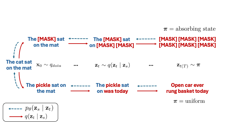
Discrete diffusion with absorbing state (top) or uniform noise (bottom) as the limiting distribution $\boldsymbol{\pi}$.

The seminal D3PM paper (Austin et al., 2021) defined a noising process over discrete data via transition matrices $Q_{t|s}$ whose $(i, j)^{\text{th}}$ entries correspond to the probability of transitioning from the $i^{\text{th}}$ state at time $s$ to the $j^{\text{th}}$ state at time $t$. This induces a Markov corruption process where we have $q(\mathbf{z}_t | \mathbf{z}_s) = \mathrm{Cat}(\mathbf{z}_t; Q_{t|s}\mathbf{z}_s)$. Sahoo et al. (2024) build off this framework to introduce specialized algorithms that are both simpler and more effective than the general D3PM framework. They focus on a specific class of forward processes from D3PM that can be defined as interpolations between clean data and a noisy prior $\boldsymbol{\pi}$, and we adopt their notation below: $$q(\mathbf{z}_t \mid \mathbf{x}_0) = \mathrm{Cat}(\mathbf{z}_t; \alpha_t\mathbf{x}_0 + (1 − \alpha_t)\boldsymbol{\pi}),$$ where $\alpha_t = \alpha(t)$ is a noise schedule monotonically decreasing in $t$. Defining $\alpha_{t|s} = \alpha_t / \alpha_s$, this class of processes admit the following posteriors $$q(\mathbf{z}_s | \mathbf{z}_t, \mathbf{x}_0) = \mathrm{Cat}\left(\mathbf{z}_s; \frac{[\alpha_{t|s} \mathbf{z}_t + (1 - \alpha_{t|s})\mathbf{1} \boldsymbol{\pi}^\top \mathbf{z}_t] \odot [\alpha_s \mathbf{x}_0 + (1 - \alpha_s) \boldsymbol{\pi}]}{\alpha_t \mathbf{z}_t^\top \mathbf{x}_0 + (1 - \alpha_t)\mathbf{z}_t^\top\boldsymbol{\pi}} \right).$$ Of note, for absorbing-state diffusion, where $\boldsymbol{\pi} = \boldsymbol{m}$, a one-hot vector at the special $\texttt{[MASK]}$ token index, Sahoo et al. (2024) show that when the latent $\mathbf{z}_t \neq \boldsymbol{m}$ then $q(\mathbf{z}_s \mid \mathbf{z}_t, \mathbf{x}_0) = \mathrm{Cat}(\mathbf{z}_s; \mathbf{z}_t)$, which reflects the fact that unasked tokens at time $t$ must remain unmasked for all time $s < t$.

Diffusion models are trained to minimize a variational upper bound (NELBO) given by: $$\mathbb{E}_q\Bigg[\underbrace{- \log p_\theta(\mathbf{x}_0 | \mathbf{z}_{t(0)})}_{\normalsize\begin{array}{c}\mathcal{L}_{recons}\end{array}} + \underbrace{\sum_{i=1}^T \mathrm{KL}[q(\mathbf{z}_{s(i)} | \mathbf{z}_{t(i)}, \mathbf{x}_0) \| p_\theta(\mathbf{z}_{s(i)} | \mathbf{z}_{t(i)})]}_{\normalsize\begin{array}{c}\mathcal{L}_{diff}\end{array}}\Bigg] + \underbrace{\mathrm{KL}[q(\mathbf{z}_{t(T)} | \mathbf{x}_0) \| p_\theta(\mathbf{z}_{t(T)})]}_{\normalsize \begin{array}{c}\mathcal{L}_{prior}\end{array}},$$ where $\mathrm{KL}$ refers to the Kullback-Leibler divergence, and the expectation is taken over the noising process. $\mathcal{L}_{prior}$ refers to the prior regularization term, which is used to ensure that the final latent $\mathbf{z}_{t(T)}$ is close to the prior distribution. $\mathcal{L}_{recons}$ is the reconstruction loss, which measures the negative log-likelihood of the clean data given the latent at time $t(0)$. Finally, $\mathcal{L}_{diff}$ is the diffusion loss, which measures the KL divergence between the noised and denoised latents.

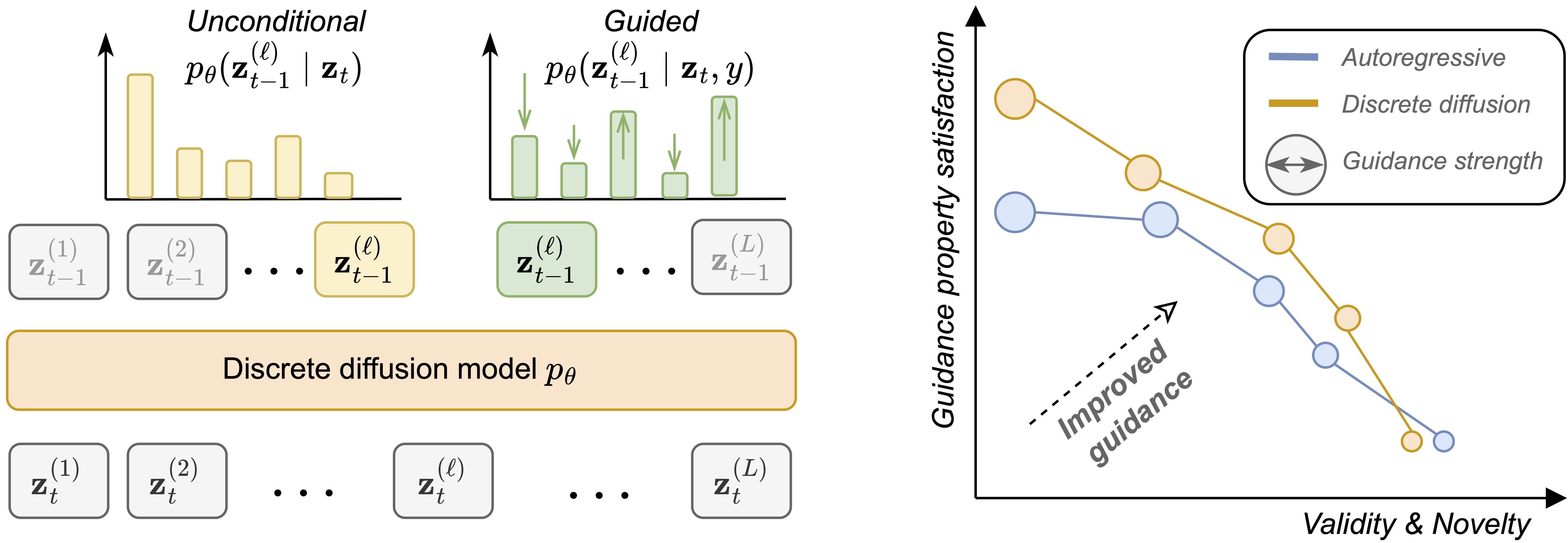
Often we model entire sequences, and not just individual tokens, which we denote as $\mathbf{x}_0^{(1:L)}$ and $\mathbf{z}_t^{(1:L)}$ for a sequences clean data and latents of length $L$, respectively. We assume that the forward noising process factorizes independently across tokens, so that the noising process for a sequence is the product of the noising processes for each token and that the denoising network, when conditioned on a sequence of latent variables, factorizes independently across tokens as well.

Why Guidance in Discrete Diffusion is Hard

Current guidance mechanisms for diffusion models rely on Langevin dynamics and computation of the gradient of the log-likelihood with respected to latent variables, as below: $$\begin{aligned}\nabla_{\mathbf{z}_s}\log(p_\theta^\gamma(\mathbf{z}_s\mid \mathbf{z}_t, y)) &= \gamma\nabla_{\mathbf{z}_s}\log(p_\phi(y\mid \mathbf{z_s})) + \nabla_{\mathbf{z}_s}\log(p_\theta(\mathbf{z_s} \mid \mathbf{z}_t)) && \text{classifier-based} \\ \nabla_{\mathbf{z}_s}\log(p_\theta^\gamma(\mathbf{z}_s\mid \mathbf{z}_t, y)) &= \gamma\nabla_{\mathbf{z}_s}\log(p_\theta(\mathbf{z}_s \mid \mathbf{z}_t, y)) + (1-\gamma)\nabla_{\mathbf{z}_s}\log(p_\theta(\mathbf{z}_s\mid\mathbf{z}_t)) && \text{classifier-free},\end{aligned}$$ where $\gamma$ is an inverese temperature parameter that controls the strength of the guidance, $y$ is the desired ouput class, $p_\theta$ is the denoising diffusion model (unconditional / conditional), and $p_\phi$ is a separate classifier model.

The reliance on the gradient computation blocks the application of these guidance mechanisms to discrete diffusion models, as the gradient of the log-likelihood with respect to the discrete latent variables is not defined.

Proposed Discrete Guidance Mechanisms

To overcome the issues of applying gradient-based guidance mechanisms to discrete diffusion models, we propose two mechanisms for discrete guidance that re-weight the probabilities assigned by the denoising model according to a $\gamma$-scaled guidance term.

Discrete Classifier-Free Guidance

First, we can achieve classifier-free guidance through a simple derivation that relies on (repeated) applications of Bayes' rule to the tempered distribution $p_\theta^\gamma(\mathbf{z}_s\mid \mathbf{z}_t, y)$. We train a conditional and unconditonal diffusion model, both of which factorize independently across tokens in a sequence in order to sample each token independently from the following distribution: $$p_\theta^\gamma(\mathbf{z}_s\mid \mathbf{z}_t, y) \propto p_\theta(\mathbf{z}_s\mid \mathbf{z}_t, y)^\gamma\cdot p_\theta(\mathbf{z}_s \mid \mathbf{z}_t)^{(1-\gamma)}.$$ That is, we sample each token from a weighted combination of the conditional and unconditional diffusion models. Since both $p_\theta(\mathbf{z}_s\mid \mathbf{z}_t, y)$ and $p_\theta(\mathbf{z}_s \mid \mathbf{z}_t)$ are modeled with independent factorization across tokens, we can sample an entire sequence as follows: $$p^\gamma_\theta(\mathbf{z}_s^{(1:L)} \mid _t^{(1:L)}, y) = \prod_{\ell=1}^{L}\frac{1}{Z^{(\ell)}}p_\theta(\mathbf{z}_s^{(\ell)} \mid \mathbf{z}_t^{(1:L)}, y)^\gamma p_\theta(\mathbf{z}_s^{(\ell)}\mid\mathbf{z}_t^{(1:L)})^{(1-\gamma)},$$ where $Z^{(\ell)} = \sum_{\mathbf{z}'_{s}}p_\theta(\mathbf{z}'_{s} \mid \mathbf{z}_t^{(1:L)}, y)^\gamma p_\theta(\mathbf{z}'_s\mid\mathbf{z}_t^{(1:L)})^{(1-\gamma)}$ is the per-token partition function.

We dub this guidance mechanism as D-CFG for Discerete Classifier-Free Guidance.

The temperature $\gamma$ controls the strength of guidance, i.e., how strongly we 'focus' on the conditional distribution. (Left) Discrete Classifier-Free Guidance We downweigh the output of an unconditional diffusion model and upweigh the output of conditional diffusion model (both of which factorize independently across a sequence) to produce a guided distribution per token. (Right) Discrete Classifier-Based Guidance We adjust the output of the unconditional model by the probability assigned by a classifier to sequences with a single token change. Our assumption that the guided distribution factorizes independently across tokens allows us to tractably compute this distribution.

Discrete Classifier-Based Guidance

Extending classifier-based guidance to diffusion models is difficult because the guiding classifier need not factorize the same as the diffusion denoising network, which would imply that the classifier needs to be evaluated on exponentially many sequence combinations. We resolve this using factorization assumptions on the decoding model and a Taylor expansion trick.

To formulate discrete classifier-based guidance, we make the assumption that conditioned on $\mathbf{z}_t^{(1:L)}$, the tempered distribution from which we want to sample $p^\gamma(\mathbf{z}_s^{(1:L)} \mid \mathbf{z}_t^{1:L}, y)$ factorizes independently across tokens. Therefore, we can focus on the tempered distirbution of each token $\mathbf{z}_s^{(\ell)},$ for $\ell \in 1,\ldots, L$: $$p^\gamma(\mathbf{z}_s^{(\ell)} \mid \mathbf{z}_t^{(1:L)}, y) \propto p(y \mid \mathbf{z}_s^{(\ell)}, \mathbf{z}_t^{(1:L)})^\gamma p(\mathbf{z}_s^{(\ell)} \mid \mathbf{z}_t^{(1:L)}).$$ In practice, we can sample from $p^\gamma(\mathbf{z}_s^{(\ell)} \mid \mathbf{z}_t^{(1:L)}, y)$ by training a classifier on noised latents $\mathbf{z}_t^{(1:L)}$ for $t \in [0, 1]$ and use this to model the first term on the right hand side by only evaluating $p_\phi$ on sequences for which $\mathbf{z}_s^{(1:L)}$ and $\mathbf{z}_t^{(1:L)}$ differ by at most the token at position $\ell$. We will define this set of sequences as $\tilde{\mathcal{Z}}_\ell(\mathbf{z_t}^{1:L}) = \{\tilde{\mathbf{z}}^{(1:L)} \mid \tilde{\mathbf{z}}^{(\ell')} = \mathbf{z_t}^{(\ell')}\text{ for all }\ell' \neq \ell\}$. We can then sample from the re-normalized distribution: $$p^\gamma_{\phi, \theta}(\mathbf{z}_s^{(\ell)} \mid \mathbf{z}_t^{(1:L)}, y) = \frac{p_\phi(y \mid \tilde{\mathbf{z}}^{(1:L)})^\gamma p_\theta(\mathbf{z}_s^{(\ell)} \mid \mathbf{z}_t^{(1:L)})}{\sum_{\tilde{\mathbf{z}}^{(1:L)}}p_\phi(y \mid \tilde{\mathbf{z}}^{(1:L)})^\gamma p_\theta(\mathbf{z}_s^{(\ell)} \mid \mathbf{z}_t^{(1:L)})}.$$ Restricting the summation in the denominator of the equation above to $\tilde{\mathcal{Z}}_\ell(\mathbf{z}_t^{(1:L)})$ makes normalization tractable.

Our method can be thought of as an adaptation of the successful FUDGE (Yang & Klein, 2021) approach, which guides AR generation, to discrete diffusion, similar to how NOS (Gruver et al., 2024) extended the AR guidance mechanism of PPLM (Dathathri et al., 2019) to diffusion models. We dub this guidance mechanism as D-CBG for Discerete Classifier-Based Guidance.

Uniform Diffusion Language Models (UDLM)

While masked diffusion models demonstrate better language modeling compared to other discrete diffusion (Austin et al. 2021; Lou et al. 2023), we argue that they are less amenable to guidance, since once a token is unmasked at some time $t$ it remains so for all $s < t$. In contrast, with uniform noising, intermediate latents can be refined multiple times throughout the denoising process. We therefore revisit categorical uniform noise discrete diffusion, where $\boldsymbol{\pi} = \boldsymbol{u} = 1/N$, where $N$ is the size of the vocabulary. Our aim is that by analyzing this class of diffusion models more carefully, we can reduce the gap to absorbing-state and yield performant models that are more easily steered by the guidance tools we developed above.

Uniform Noise Forward Process We formulate uniform noise diffusion using the interpolating discrete diffusion framework (Sahoo et al. (2024)). When letting $\boldsymbol{\pi} = \boldsymbol{u}$, the input $\mathbf{x}$ transitions to a random state with some probability at each time step. Crucially, after $\mathbf{x}$ changes once, it can do so again. Formally, when $\boldsymbol{\pi} = \boldsymbol{u}$, the posterior from above becomes $$q(\mathbf{z}_s \mid \mathbf{z}_t, \mathbf{x}_0) = \mathrm{Cat} \left(\mathbf{z}_s;\frac{N \alpha_t \mathbf{z}_t \odot \mathbf{x}_0 + (\alpha_ts - \alpha_t)\mathbf{z}_t + (\alpha_s - \alpha_t)\mathbf{x}_0 + \frac{(\alpha_s - \alpha_t)(1- \alpha_s)}{N \alpha_s}\boldsymbol{1}}{N \alpha_t\langle \mathbf{z}_t, \mathbf{x}_0\rangle + 1 - \alpha_t}\right)$$ Denoising Process The optimal form for the reverse diffusion process $p_\theta$ matches the posterior. In fact, setting $p_\theta$ to the posterior reduces the KL terms in the ELBO to zero. However, setting $p_\theta$ to exactly the posterior is not possible because it cannot be a function $\mathbf{x}_0$ (which $p_\theta$ is generating). Therefore, we introduce a predictive model of the 'clean' data given a noisy latent $\mathbf{z}_t$ at time $t$. We use $\mathbf{x}_\theta$ to parameterize the denoising process as $p_\theta(\mathbf{z}_s \mid \mathbf{z}_t) = q(\mathbf{z}_s \mid \mathbf{z}_t, \mathbf{x} = \mathbf{x}_\theta)$, yielding: $$p_\theta(\mathbf{z}_s \mid \mathbf{z}_t) = \mathrm{Cat} \left(\mathbf{z}_s;\frac{N\alpha_t \mathbf{z}_t \odot \mathbf{x}_\theta + (\alpha_ts - \alpha_t)\mathbf{z}_t + (\alpha_s - \alpha_t)\mathbf{x}_\theta + \frac{(\alpha_s - \alpha_t)(1- \alpha_s)}{N\alpha_s}\boldsymbol{1}}{N \alpha_t\langle \mathbf{z}_t, \mathbf{x}_\theta\rangle + 1 - \alpha_t}\right).$$ Note that this minimizes the $\mathcal{L}_{diff}$ precisely when $\mathbf{x}_\theta = \mathbf{x}_0,$ as desired.

UDLM To build towards Uniform Discrete Language Models (UDLM), we derive an improved variational objective by taking $T\rightarrow\infty$ and analyzing each term $\mathcal{L}_{recons}, \mathcal{L}_{diff}, \mathcal{L}_{prior}$, introduced above. This yields three improvements: (1) a simple and elegant closed-form expression for the variational bound that is easier to reason about; (2) an analytical reduction of $\mathcal{L}_{recons}, \mathcal{L}_{prior}$ to zero, which tightens the ELBO; (3) a further tightening via the continuous-time extension of $\mathcal{L}_{diff}$. Please refer to our manuscript for more details about this derivation.

Experiments

Language Modeling Results

Our language modeling experiments reveal that (1) contrary to a widely-held belief, uniform noise diffusion can attain state-of-the-art performance on small vocabulary datasets , and that (2) our UDLM is state-of-the-art among uniform noise diffusion models.

UDLM performs best in smaller vocabulary regimes. Values correspond to perplexity (PPL; $\downarrow$) on various datasets. Best values are **bolded.**
Domain	Dataset	Vocab. size	AR	MDLM	UDLM
Bio	Species-10	12	2.88	3.17$_{\geq}$	3.15$_{\geq}$
Chem	QM9	40	2.19	2.12$_{\geq}$	2.02$_{\geq}$
Images	CIFAR-10	256	-	9.14$_{\geq}$	11.21$_{\geq}$
NLP	text8	35	2.35	2.62$_{\geq}$	2.71$_{\geq}$
	Amazon	30,522	21.67	24.93$_{\geq}$	27.27$_{\geq}$
	LM1B	30,522	22.32	27.04$_{\geq}$	31.28$_{\geq}$

*UDLM outperforms previously reported uniform noise discrete diffusion models on natural language text datasets. Best values are **bolded**.*
Dataset	D3PM Uniform	SEDD Uniform	UDLM
text8 (BPC $\downarrow$)	1.61	1.47	1.44
LM1B (PPL $\downarrow$)	77.59	40.25	31.28

Guidance Results

Our guidance results indicate that (1) classifier-free guidance is more useful when paired with diffusion models compared to AR and that (2) our proposed D-CBG is the best classifier-based method for discrete guidance, especially when combined with UDLM.

Species-specific Genome Generation: We train on the reference genomes of ten diverese species using sequences of 32,768 base pairs. We then generate novel sequences using the trained models conditioned on the species label. As quality measures for each species class, we compute the Jensen-Shannon (JS) distance between the $k$-mer frequencies of the generated sequences and those from the validation set, and report the mean JS across species (weighted by species frequency in the dataset), with smaller values indicating better $k$-mer distributional overlap between the ground truth and generated sequences. Additionally, we train a small classifier to distinguish between generated and validation set sequences and report the area under the receiver operator curve for this classifier (Disc. AUROC). Values closer to 0.5 indicate that the classifier is unable to distinguish between synthetic and true sequences. To measure the controllability, we train a separate classifier on this dataset and measure macro F1 score of this oracle classifier on the generated sequences. For reference, we also provide metrics for randomly generating sequences with nucleotide frequencies proportional to species representation in the data.

We find that both MDLM and UDLM are able to better generate sequences that match the desired control parameter, with higher F1 scores relative to AR. Moreover, UDLM is able to outperform MDLM in satisfying this control. Importantly, we find that only UDLM is amenable to increasing the guidance parameter $\gamma$, where its metrics improves while AR and MDLM metrics degrade. Finally, of note, the diffusion model generation for this experiment is accomplished with far fewer function evaluations compared to AR. Whereas AR must decode each of the 32,768 tokens, because MDLM and UDLM can decode multiple tokens in parallel, we generate with $T = 512$.

*Diffusion decoding with D-CFG is more controllable than AR for genomic sequences. Best values are **bolded**.*
Model	Guidance	3-mer JS ($\downarrow$)	6-mer JS ($\downarrow$)	Disc. AUROC ($\uparrow$)	Oracle F1 ($\uparrow$)
Random	N/A	0.13	0.22	1.00	0.07
AR	D-CFG$_{\gamma=1}$	0.03	0.07	0.53	0.87
AR	D-CFG$_{\gamma=2}$	0.05	0.12	0.90	0.81
AR	D-CFG$_{\gamma=3}$	0.07	0.15	0.97	0.74
MDLM	D-CFG$_{\gamma=1}$	0.02	0.06	0.51	0.88
MDLM	D-CFG$_{\gamma=2}$	0.05	0.11	0.74	0.91
MDLM	D-CFG$_{\gamma=3}$	0.11	0.20	0.93	0.78
UDLM	D-CFG$_{\gamma=1}$	0.02	0.06	0.52	0.91
UDLM	D-CFG$_{\gamma=2}$	0.05	0.13	0.61	0.93
UDLM	D-CFG$_{\gamma=3}$	0.08	0.20	0.87	0.94

Molecule Property Maximization: We use the small molecule QM9 dataset to investigate novel generation of sequences that maximize some property, either drug-likeness (QED) or a count of the number of rings present in the molecule. Our goal is to explore which models and guidance mechanisms best trade-off sample quality and control. We only report values for which we generated at least 50 novel sequences (out of 1,024). In the figure below, we see that our guidance mechanisms enable diffusion generation that better trades-off sample novelty with guidance property satisfaction.

Diffusion models extend the steer-ability Pareto frontier compared to AR. (Left) Comparing D-CBG and FUDGE for maximizing the drug-likeness (QED) property in the QM9 dataset. Using our D-CBG outperforms FUDGE classifier guidance for AR. Only UDLM can accommodate larger $\gamma$ values that enable better molecule property maximization. (Right) Comparing D-CFG for diffusion and AR models for maximizing ring-count in the QM9 dataset. Diffusion models better trade-off novel generation and property maximization.

Class-conditional Image Generation: We train discrete diffusion models on a discretized version of the CIFAR10 dataset. We then conditionally generate images (with and without classifier-free guidance). In the tables below on the left, we see that both MDLM and UDLM outperform finite-time counterparts (in the form of D3PM) with improved image quality metrics of Frechet inception distance (FID) and Inception Score (IS). This is especially true when we add guidance using D-CFG. Additionally, on the right table, we explore faster inference settings (smaller $T$ ) where diffusion models predict multiple pixels in parallel. MDLM's performance deteriorates with smaller $T$, whereas UDLM is robust to this setting. This validates a key motivation behind UDLM: in settings where MDLM 'locks in' certain predictions that it cannot change, UDLM is more resilient given that all tokens can change throughout the decoding process.

Guidance improves quality on discretized CIFAR10. FID and IS for finite- (D3PM) and continuous-time (MDLM / UDLM) discrete diffusion models. Guidance using D-CFG ($\gamma=4$). Best values are **bolded**.
Model	FID ($\downarrow$)	IS ($\uparrow$)
D3PM Absorb	41.28	6.26
MDLM	33.75	6.74
MDLM D-CFG	15.56	9.02
D3PM Uniform	51.27	5.99
UDLM	33.65	6.86
UDLM D-CFG	23.21	8.66

UDLM is robust to faster sampling. Images sampled from a conditional model (D-CFG$_{\gamma=1}$) trained on CIFAR10. F1 metric from a separate classifier trained to identify class label used for generation. Best metric per $T$ is **bolded**.
Model	FID ($\downarrow$)	IS ($\uparrow$)	F1 ($\uparrow$)
$T=128$
MDLM	64.09	5.81	0.63
UDLM	30.48	7.30	0.80
$T=1024$
MDLM	27.94	7.13	0.81
UDLM	26.70	7.43	0.81

Conclusion

In search of a more controllable diffusion process, in this work, we derived a tight variational bound for uniform noise discrete diffusion, closing the gap to state-of-the-art absorbing-state diffusion models. We also highlighted that contrary to previous findings, in small vocabulary regimes, uniform noise is on par or better than absorbing state. We then demonstrated that straightforward adaptations of classifier-based and classifier-free guidance can offer improved guided generation relative to AR models. We found that with classifier-free mechanisms, diffusion models are more amenable to control without sacrificing quality of generated sequences. We also demonstrated that our classifier-based method is better than previous ones for both AR and diffusion models.

BibTeX


        @article{schiff2024discreteguidance,
          title={Simple Guidance Mechanisms for Discrete Diffusion Models},          
          author={Schiff, Yair and Sahoo, Subham Sekhar and Phung, Hao and Wang, Guanghan and Boshar, Sam and Dalla-torre, Hugo and de Almeida, Bernardo P and Rush, Alexander and Pierrot, Thomas and Kuleshov, Volodymyr},
          journal={arXiv preprint arXiv:2412.10193},
          year={2024}
        }

Dataset	D3PM Uniform	SEDD Uniform	UDLM
text8 (BPC \(\downarrow\))	1.61	1.47	1.44
LM1B (PPL \(\downarrow\))	77.59	40.25	31.28

Model	FID (\(\downarrow\))	IS (\(\uparrow\))	F1 (\(\uparrow\))
\(T=128\)
MDLM	64.09	5.81	0.63
UDLM	30.48	7.30	0.80
\(T=1024\)
MDLM	27.94	7.13	0.81
UDLM	26.70	7.43	0.81

Simple Guidance Mechanisms forDiscrete Diffusion Models